Let's talk about qex.
I have been building a small language for expressing quant alphas, the cross-sectional forecasts a systematic investor turns into a portfolio. It is called qex, which is short for "quantitative expression" and which I pronounce as kecks. The project is open source, and there is a dedicated documentation site. A simple but mighty one-line qex expression is:
rank(-returns(20) / volatility(60))That says to rank stocks by risk-adjusted one-month momentum and bet against the winners, which makes it a mean-reversion alpha, and the equivalent pandas is fifty lines of rolling windows, axis arguments, and NaN handling. You do not need to be a programmer to read the short version: most portfolio managers can code, but anyone who can write an Excel formula can read that line, and most of what follows.
That is the idea behind qex: the shortest possible distance between "I think markets behave like this" and code that tests it. The belief goes in, nearly word for word, and nothing else does.
Sidebar: The cross-section. Working across a wide cross-section
of stocks at once is second nature inside institutional quant firms and
somewhat obscure outside them. The motivation is Grinold's Fundamental Law
of Active Management: the information ratio is roughly the skill of each
forecast, the information coefficient, times the square root of breadth,
the number of independent bets, or IR = IC * sqrt(BR).
Institutional quants exploit small mispricings, so each forecast carries
little skill, and the way to turn that into a meaningful risk-adjusted
return is to apply it across the largest breadth of opportunities
possible. A broad universe also guards against selecting your way into a
flattering sample.
From a belief to a line
Here is a belief about markets, built up one clause at a time, and the expression built up alongside it.
# Stocks that fell last week bounce back.
rank(-returns(5))

# ...relative to their sector,
group_demean(rank(-returns(5)), 'sector')

# ...measured in units of how much the stock usually moves,
group_demean(rank(-returns(5) / volatility(60)), 'sector')

# ...and I do not want to trade every wiggle.
decay_linear(group_demean(rank(-returns(5) / volatility(60)), 'sector'), 10)
Each clause of the sentence is one operator, and the expression never says anything the sentence does not. Other beliefs read the same way:
# Past-year winners keep winning, skipping the last month.
rank(delay(returns(231), 21))

# Quiet stocks beat noisy ones.
rank(-volatility(252))

# When price and volume move together, the move fades.
rank(-ts_corr(returns(1), volume(1), 20))

# Momentum, but only in names that trade $10M a day.
rank(returns(20)) * (adv(20) > 10000000)

# Earnings surprises keep drifting for a quarter.
rank(fill_forward(field('earnings_actual') - field('earnings_estimate'), 60))
What is missing is everything a pandas version would add: the loops, the
index alignment, the axis= arguments, the warmup, the NaN handling, the
care not to peek at tomorrow. None of it is the belief, all of it is where
the bugs live, and in qex it is the engine's job, written once. The mental
load left is the idea itself.
Why a language
Anyone who has read Kakushadze's 101 Formulaic Alphas will
recognize the style.
Expressions like rank(ts_corr(returns(1), volume(1), 20)) are
indicative of one flavor of domain-specific language, or DSL, that
large quant shops could use to describe alphas.
The usual argument for the form is readability, and it is true that the expression captures the idea where the pandas buries it. But in the age of coding agents, "a human has to read this" gets weaker every month, because nobody reads the fifty lines any more; a model writes them and another model reviews them. Readability for the reviewer matters less than it used to. Writability for the person with the idea, the short path from a belief to a test, matters more than ever, and so does what a closed language changes for the machines. The real case for a language is about both:
- The expression is the hypothesis, not the implementation. It is the smallest artifact that fully specifies an alpha, and everything else is engine, which is written once.
- A closed vocabulary makes generated work checkable. When an agent writes fifty lines of pandas, a lookahead, a misaligned index, or a wrong axis can hide on any line, and reviewing it costs about what writing it did. When an agent writes a qex expression, every well-formed expression is already aligned, warmup-aware, and lookahead-free, so the only thing it can be wrong about is the idea.
- Terse is cheap for models. An expression is a few dozen tokens where the pandas is a few thousand, which matters when you want a model to propose, mutate, and score thousands of candidates, or hold an entire alpha library in context while it works.
- Alphas become data. Expressions can be stored, diffed, deduplicated, searched, and evolved. Shared sub-expressions are visible, so a thousand alphas cost far less than a thousand times one. None of that is possible when each alpha is its own script.
- The grammar is a search space. Machine-generated alphas need somewhere to search, and "all Python programs" is not it. A closed set of operators and fields, composed by a grammar, is a finite and well-shaped space: every point in it is a valid alpha, neighbors are a single operator or window away, and mutation and crossover are defined. That is what genetic programming and reinforcement learning over alphas have always needed, and what a pile of scripts never gives them.
- Review is constant time. A portfolio manager can audit the intent of an expression at a glance, and that is the only kind of review that scales to machine-generated research.
In the last post I described the quant workflow as an assembly line, with alpha research as one stage feeding signal combination downstream. An alpha language is the interface between those two stages, and it is what lets alpha research be done by many people, or by many agents, and still plug into the same pipeline.
Three axes
A dataset, e.g., pricing, is organized in qex as tickers across the columns and dates down the rows. Every operation in qex works along one of three axes, and knowing which one is most of what you need to read an expression.
The easiest way to see them is on a dataset small enough to check by hand.
Here are the actual closing prices, close(), of five stocks over six
trading days in March 2025:
| close() | AAPL | MSFT | XOM | CVX | JPM |
|---|---|---|---|---|---|
| Mar 3 | 238.03 | 388.49 | 107.76 | 153.09 | 260.62 |
| Mar 4 | 235.93 | 388.61 | 107.54 | 152.00 | 250.25 |
| Mar 5 | 235.74 | 401.02 | 105.44 | 150.81 | 251.53 |
| Mar 6 | 235.33 | 396.89 | 107.62 | 152.95 | 246.54 |
| Mar 7 | 239.07 | 393.31 | 109.02 | 156.34 | 242.28 |
| Mar 10 | 227.48 | 380.16 | 111.80 | 157.57 | 232.22 |
The three CVX closes in bold are the ones averaged in the first example below.
Time series operations run down each column, one ticker at a time.
ts_mean(close(), 3)| ts_mean(close(), 3) | AAPL | MSFT | XOM | CVX | JPM |
|---|---|---|---|---|---|
| Mar 3 | – | – | – | – | – |
| Mar 4 | – | – | – | – | – |
| Mar 5 | 236.57 | 392.71 | 106.91 | 151.97 | 254.13 |
| Mar 6 | 235.67 | 395.51 | 106.87 | 151.92 | 249.44 |
| Mar 7 | 236.71 | 397.07 | 107.36 | 153.37 | 246.78 |
| Mar 10 | 233.96 | 390.12 | 109.48 | 155.62 | 240.35 |
CVX on March 5 is the average of its last three closes, the three in bold
above: (153.09 + 152.00 + 150.81) / 3 = 151.97. No other stock enters into it. The first two rows are empty because
there are not yet three days to average; that warmup is the engine's job, not
yours. The same goes for every ts_ operator:
ts_mean(close(), 20)      # 20-day rolling mean
delta(close(), 5)         # change over 5 days
ts_corr(returns(1), volume(1), 20)
ewma(returns(1), 10)      # exponential average, 10-day half-life
Cross-sectional operations run across each row, one day at a time. Start
with each stock's daily return, returns(1), here in percent. March 3 is
empty, since a return needs the previous day's close:
| returns(1) | AAPL | MSFT | XOM | CVX | JPM |
|---|---|---|---|---|---|
| Mar 3 | – | – | – | – | – |
| Mar 4 | −0.88 | +0.03 | −0.20 | −0.71 | −3.98 |
| Mar 5 | −0.08 | +3.19 | −1.95 | −0.78 | +0.51 |
| Mar 6 | −0.17 | −1.03 | +2.07 | +1.42 | −1.98 |
| Mar 7 | +1.59 | −0.90 | +1.30 | +2.22 | −1.73 |
| Mar 10 | −4.85 | −3.34 | +2.55 | +0.79 | −4.15 |
Then rank them across the stocks on each day:
rank(returns(1))| rank(returns(1)) | AAPL | MSFT | XOM | CVX | JPM |
|---|---|---|---|---|---|
| Mar 3 | – | – | – | – | – |
| Mar 4 | 0.4 | 1.0 | 0.8 | 0.6 | 0.2 |
| Mar 5 | 0.6 | 1.0 | 0.2 | 0.4 | 0.8 |
| Mar 6 | 0.6 | 0.4 | 1.0 | 0.8 | 0.2 |
| Mar 7 | 0.8 | 0.4 | 0.6 | 1.0 | 0.2 |
| Mar 10 | 0.2 | 0.6 | 1.0 | 0.8 | 0.4 |
rank returns each stock's percentile within the day, between 0 and 1: with
five stocks the ranks are 0.2, 0.4, 0.6, 0.8 and 1.0, from the lowest value
to the highest, and with two thousand stocks they fill the interval almost
evenly. March 10 was a sharp sell-off in technology stocks. AAPL had the
worst day of the five, −4.85%, so it ranks 0.2, and XOM the best, +2.55%, so
it ranks 1.0. Each row is ranked on its own; yesterday plays no part.
A rank throws away the size of the moves and keeps their order, which is why
it is the usual first step of an alpha: one huge outlier cannot dominate the
book. Other cross-sectional operators:
rank(returns(20))         # percentile rank across stocks, 0 to 1
zscore(returns(20))
winsorize(returns(20), 0.05)
Group operations are cross-sectional within a bucket, such as a sector, an industry, or a pair. AAPL and MSFT are Technology, XOM and CVX are Energy, and JPM is Financials:
group_demean(returns(1), 'sector')| group_demean(…) | AAPL | MSFT | XOM | CVX | JPM |
|---|---|---|---|---|---|
| Mar 3 | – | – | – | – | – |
| Mar 4 | −0.46 | +0.46 | +0.25 | −0.25 | 0.00 |
| Mar 5 | −1.64 | +1.64 | −0.58 | +0.58 | 0.00 |
| Mar 6 | +0.43 | −0.43 | +0.32 | −0.32 | 0.00 |
| Mar 7 | +1.25 | −1.25 | −0.46 | +0.46 | 0.00 |
| Mar 10 | −0.75 | +0.75 | +0.88 | −0.88 | 0.00 |
On March 10 Technology fell 4.10% on average, so AAPL, down 4.85%, was 0.75% worse than its sector, and MSFT, down 3.34%, 0.75% better. Energy rose 1.67%, so XOM, up 2.55%, was 0.88% ahead of it and CVX 0.88% behind. JPM, alone in its sector, is always zero. What is left is how each stock did against its peers, which is what a sector-neutral book bets on. Other group operators:
group_demean(returns(60) / volatility(60), 'sector')   # sector-neutral momentum
group_rank(returns(20), 'industry')
They compose, so sector-neutral momentum restricted to liquid names is:
group_demean(rank(returns(20)) * (adv(20) > 1000000), 'sector')When an expression repeats itself, let names the pieces:
let mom    = returns(60),
    vol    = volatility(60),
    sharpe = mom / vol
in rank(sharpe) * sign(mom)
The full list of operators, with what each one does, is in the qex docs' All Operations reference.
From a signal to a book
An alpha's output is a score for every stock on every day. To trade it, the scores have to become portfolio weights, and the standard book for this kind of research is dollar-neutral, as many dollars long as short, with a gross of one, so the absolute weights add up to one dollar. Two cross-sectional operators do it:
scale(demean(rank(returns(1))))Here it is on the March 10 ranks from above:
| March 10 | rank | demean | scale = weight |
|---|---|---|---|
| AAPL | 0.2 | −0.4 | −0.333 |
| MSFT | 0.6 | 0.0 | 0.000 |
| XOM | 1.0 | +0.4 | +0.333 |
| CVX | 0.8 | +0.2 | +0.167 |
| JPM | 0.4 | −0.2 | −0.167 |
| sum | 3.0 | 0.0 | 0.000 |
| sum of absolute values | 3.0 | 1.2 | 1.000 |
demean subtracts the day's average rank, 0.6, so the scores sum to zero:
that is the dollar neutrality. scale divides by the sum of the absolute
values, 1.2, so they sum to one: that is the gross of one. The book is long
XOM 33.3% and CVX 16.7%, short AAPL 33.3% and JPM 16.7%, and flat MSFT, which
is 50 cents long and 50 cents short for each dollar of gross. This one buys
yesterday's winners; a minus sign in front of rank turns it into a
reversal book. Swap demean for group_demean(…, 'sector') and the book is
sector-neutral as well. Every return quoted on gross market value, or GMV,
later in this post is per dollar of exactly this kind of book.
Lazy trees, no lookahead
Parsing an expression builds a tree, and nothing is computed until you
call evaluate with data, which is a dictionary of DataFrames, one per
field, with dates down the index and tickers across the columns.
Rank
 └── Returns(period=20)
      └── Field('close')
Because the engine owns every operator, it can enforce things that are
hard to enforce in free-form pandas. The one I care most about is that
every operation looks backward, so there is no way to write an
expression that peeks at tomorrow, and delay refuses a negative period
rather than silently producing a backtest that is too good to be true.
Sparse data is a first-class case
Earnings arrive quarterly, so a DataFrame of earnings has a value on announcement day and NaN everywhere else, and ordinary rolling operations do the wrong thing on it. For that case qex has event-aware operators that roll over the past N observations rather than the past N days.
Post-earnings announcement drift, with a textbook standardized unexpected earnings score, is three lines:
let surprise = field('earnings_actual') - field('earnings_estimate'),
    sue      = surprise / ts_std_events(surprise, 8)
in rank(fill_forward(sue, 60)) - 0.5
That divides this quarter's surprise by the standard deviation of the last eight surprises, holds it for a quarter, ranks across stocks, and centers for long-short, and the expression reads like the paper.
Shared work is done once
A research session evaluates many signals, and they often have overlapping atomic units. For example, momentum, risk-adjusted momentum, and short-term reversal all need daily returns. qex builds a single graph for a set of signals and computes each unique sub-expression one time.
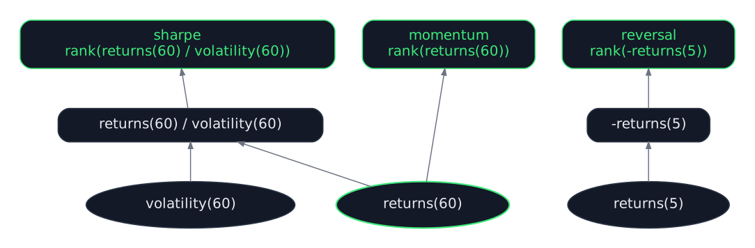
For three toy signals the saving is one node, but a portfolio may contain thousands of signals. These signals often draw from a common vocabulary of primitives. The same graph can be handed to Dask and evaluated across a cluster, with the data scattered to workers once.
Evaluation
A signal is only interesting once you know whether it predicts anything, so the package ships with the usual tooling: a long-short backtest with transaction costs and drawdown analysis, quantile analysis with rank IC, and walk-forward splits.
from qex import qex, Backtest, QuantileAnalysis

signal = qex("rank(returns(60)) - 0.5")

Backtest(signal, transaction_cost=0.001).run(data).summary()
QuantileAnalysis(signal, n_quantiles=5).run(data).summary()
There is also a multi-factor risk model whose factor definitions are themselves qex expressions, so a factor is just another signal.
A real run
Let's work some real data and an alpha idea motivated by an alpha well known in "the literature." The universe is every current S&P 500 member with a full price history back to mid-2009, 414 names, with adjusted daily bars from Yahoo Finance. Using current membership makes the basket survivorship-biased, of course. At worst, the names that fell out of the index on the way down are exactly the ones a reversal alpha would have been buying. This post is primarily about the qex machinery; your actual data should include dead stocks.
The alpha is short-term reversal, which is the family that shows up in price-only data at a horizon of days to weeks, and the economic story behind it is old and well documented. Jegadeesh (1990) and Lehmann (1990) showed that last week's losers beat last week's winners, and the standard explanation is liquidity provision: when someone has to sell in size, the price moves more than the news justifies, and whoever takes the other side is paid for it as the price comes back. Nagel (2012) makes that precise by showing that the return to reversal is compensation for supplying liquidity and spikes exactly when liquidity evaporates. It is also the alpha style in Khandani and Lo's What Happened to the Quants in August 2007?, which uses Lehmann's contrarian rule, long recent losers and short recent winners in proportion to their move, as the canonical statistical arbitrage strategy. Demeaning within sector rather than against the market is a modern refinement. This is a "poor man's residual reversal": what you want to fade is the stock-specific move and not the industry's.
In this post we capture the reversal idea as a function of where the stock closed within its own five-day high-low range (inverted so that a close near the low is a buy). It is reversal scaled by the stock's own recent volatility. Technical analysis is often derided, rightly so in most cases, because technicians don't think cross-sectionally. Here, though, they are vindicated. Technicians have called this alpha Williams %R or a stochastic oscillator for fifty years. We enhance it with the basics of the modern stat arb toolkit: rank it across stocks, demean within sector so the book is sector-neutral and dollar-neutral by construction, and smooth it with a linear decay:
let lo   = ts_min(low(), 5),
    hi   = ts_max(high(), 5),
    pos  = (close() - lo) / (hi - lo),
    book = group_demean(rank(-pos), 'sector')
in scale(decay_linear(book, 10))
pos is where the close sits in the stock's five-day range, 0 at the low and
1 at the high, so ranking -pos buys the stocks that closed near their lows
and sells the ones that closed near their highs. group_demean already makes
the book dollar-neutral, and the decay, an average of neutral days, keeps it
so; scale sets the gross to one.
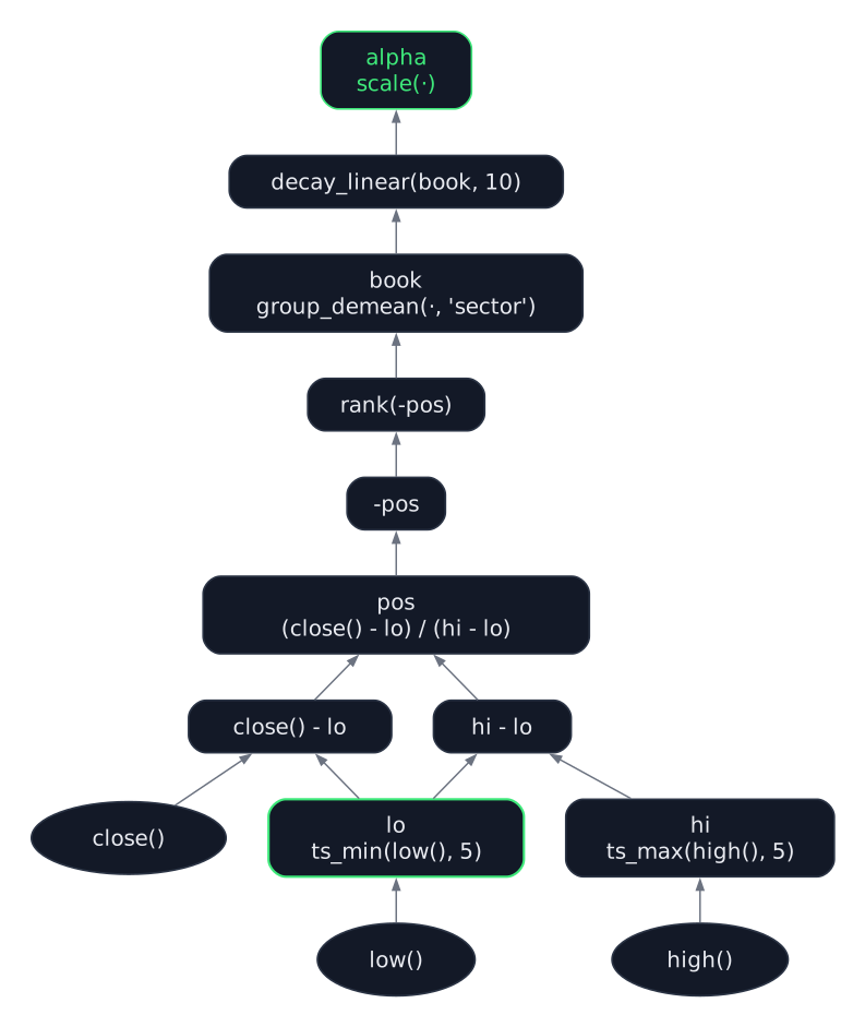
lo, is computed once and used twice.The decay is a denoiser. decay_linear is a weighted moving average whose
weights fall off linearly with age, the linear cousin of an
exponentially weighted average: over a ten-day window today carries 18%
of the weight, yesterday 16%, and the tenth day back under 2%, so the
signal is smoothed without being lagged the way an equal-weight ten-day
mean would lag it. In my experience, the decay operator is extremely powerful!
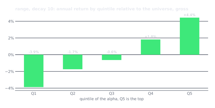
The first check, before any backtest, is whether the alpha sorts returns
at all. QuantileAnalysis cuts the universe into quintiles of the alpha
each day and holds each quintile as an equal-weight portfolio for a day.
The chart shows each quintile's return relative to the equal-weight
universe. The quintiles are monotonic, and the top-minus-bottom spread
is 8.3% a year at a Sharpe of 0.84 before costs, which is about 4% on
GMV and in line with the backtest below.
The book is rebalanced every day to the alpha's weights, and turnover is quoted per day. The run is July 2010 to December 2025. Costs are charged per unit of turnover at 2 basis points, which is an aspirational but reasonable level for an institution (I'm assuming a lot here!). All returns are on gross market value, GMV, unlevered, meaning a dollar long against a dollar short with no financing and no leverage.
One more disclosure: this is a delay-0 alpha. The signal is computed from the close and the book is traded at that same close, so the run assumes you can measure the day's range and execute on it in the same print. That is possible, with the trade computed from the closing auction's imbalance or in the last minutes before the bell, but it is not the usual setup for a high-capacity book, which computes the signal at the close and trades the next day, a delay-1 alpha. Short-horizon reversal is exactly the kind of alpha that gives something up to a day of delay, so treat these numbers as the delay-0 upper end.
The table shows the same alpha unsmoothed and with a ten-day decay.
| Range, daily | Turnover / day | Gross on GMV | Gross Sharpe | Net on GMV at 2 bps | Net Sharpe | Max drawdown |
|---|---|---|---|---|---|---|
| no smoothing | 84% | +3.8% | 0.98 | -0.5% | -0.13 | -21% |
| decay 10 | 32% | +3.8% | 0.90 | +2.2% | 0.52 | -15% |
Returns are annual and on GMV. Max drawdown is on the book net of 2 basis points.
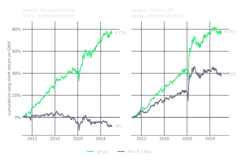
The alpha looks "ok". Gross Sharpe is 0.90 to 0.98 over the run, and the same held on a mid-cap universe and in the sub-periods I checked along the way. Just under four percent a year on the gross book is good for a single price-based alpha, since a real quant book runs at four to six times leverage, where it is mid-teens to twenty percent before financing, and no quant book trades a single alpha anyway; this one would be one input among many.
Something surprising: smoothing is close to a free lunch here. The ten-day decay cuts turnover from 84% to 32%, cuts the drawdown from 21% to 15%, takes the net Sharpe at 2 basis points from negative to about 0.5, and gives up nothing in gross return. The only cost is a tenth of a point of gross Sharpe. Diversification is supposed to be the only free lunch in finance, and smoothing a fast alpha is a close second. The reason it is nearly free is the horizon of the alpha. The chart shows the rank IC of each signal against the cumulative return over the next k days. Against the next day's return the unsmoothed signal's IC is about 0.010 and the smoothed signal's is half that, but by a week out the two curves have met, and against the next ten days they are the same, 0.011 and 0.010.
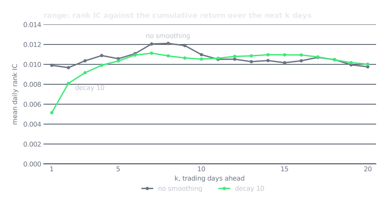
The signal predicts a move that plays out over about two weeks, so
averaging the last ten days of ranks keeps the forecast and discards the
daily noise that was driving the turnover; the smoothed ranks have a
day-to-day autocorrelation of 0.95 against 0.57 unsmoothed. The lunch
stops being free when the alpha's horizon is shorter than the smoothing
window, which is the thing to check before turning the decay up. In the
language, the check is one decay_linear around the expression and a
rerun. Turnover around thirty percent a day
is the classic mid-frequency statistical arbitrage space, ten days is a
common default for this kind of smoothing.
Who earns the gross column? Anyone who does not pay the cost. A market maker is paid the spread rather than charged it, so to a market maker the unsmoothed signal, with a gross Sharpe near one and 84% daily turnover, is not too expensive to trade; it is information to lean its quotes on. That is one way to read the move of high-frequency firms into statistical arbitrage, such as Hudson River Trading now holding positions for days and weeks (Bloomberg, December 2025): the edge is as much in what it costs to trade as in the signal. A bank desk that crosses client orders internally, or a large manager that crosses its own flow, sits in between, trading cheaply enough to keep more of the gross line.
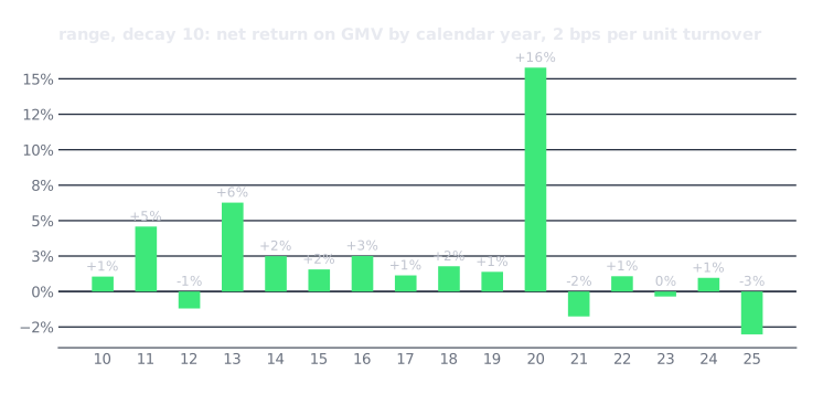
The smoothed book is positive in twelve of the sixteen full calendar years, and the standout is 2020, when reversal made in one year what it normally makes in five, which is Nagel's point exactly: dislocation is when liquidity providers get paid. The last few years are thinner, and the plain reading is that an alpha this simple decays as more capital trades it. This post is not meant to hand you a new alpha source; if it were still a secret I would not be writing it up 😉. A fun thought experiment, though, is that this approach was just as well known before 2020, and it still made five years of return in one when liquidity disappeared. Being crowded did not stop it from paying when the paying mattered.
Limitations
The data model is a single value per cell, so qex is not point-in-time on its own. If a company reports a dollar of earnings in January and restates it to three dollars in March, qex only knows one of those numbers, and the run above uses today's adjusted prices and today's index membership, which is why it is survivorship-biased. Bi-temporal data, where every value carries both the date it describes and the date it became known, could come in a future release. qex is meant in its current form as an exploration tool, not production ready for an institution.
Future directions
qex is a natural fit for a language model that writes alphas. A model that writes pandas can introduce lookahead without seeing it, and the result is fifty lines nobody wants to audit. A model that writes qex cannot look ahead, because the operators do not allow it, and the search space is constrained to a closed vocabulary of operators and fields, which makes a candidate alpha cheap to generate, cheap to check, and cheap to compare against the library. Using qex, you can ensure the agent doesn't have read access to the data directly. The package already lets a dataset describe its own fields, so an agent can discover what is available before it proposes an expression.
qex is at version 0.3, Apache licensed, and installs from the repo. Issues and pull requests are welcome.
References
- Doherty, K. "More Risk, Less Speed: Hudson River Mints Billions Slowing Down." Bloomberg, December 2025. news.bloomberglaw.com
- Grinold, R. C. "The Fundamental Law of Active Management." Journal of Portfolio Management 15(3), 1989.
- Grinold, R. C. and Kahn, R. N. Active Portfolio Management: A Quantitative Approach for Producing Superior Returns and Controlling Risk, 2nd ed. McGraw-Hill, 2000.
- Jegadeesh, N. "Evidence of Predictable Behavior of Security Returns." Journal of Finance 45(3), 1990.
- Kakushadze, Z. "101 Formulaic Alphas." Wilmott 2016(84), 2016. arxiv.org/abs/1601.00991
- Khandani, A. E. and Lo, A. W. "What Happened to the Quants in August 2007?" Journal of Investment Management 5(4), 2007. web.mit.edu/~alo
- Larkin, J. qex: a domain-specific language for quant alphas. github.com/marketneutral/alpha-parser
- Lehmann, B. N. "Fads, Martingales, and Market Efficiency." Quarterly Journal of Economics 105(1), 1990.
- Nagel, S. "Evaporating Liquidity." Review of Financial Studies 25(7), 2012.
- Tulchinsky, I. et al. Finding Alphas: A Quantitative Approach to Building Trading Strategies, 2nd ed. Wiley, 2019.